5.23. Graph (media-object)

5.23.1. Attributes

5.23.2. Description

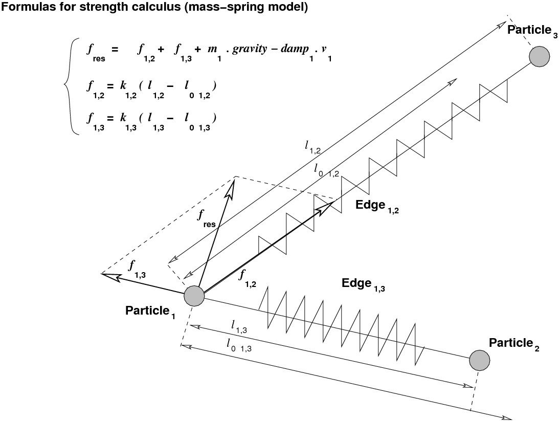
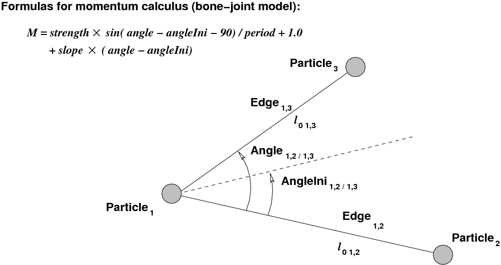
This element defines a graph of physically connected particles. Each connection is an edge of the graph and is named after the indices of the particles at its extremities. If the graph is a mass-spring model, the physical connections represent springs. The strength of a spring is proportional to the signed difference between its current length and its initial length. If the graph is a bone-joint model, the momentum of the strength applied to a joint that connects pair of edges with a common particle is proportional to the signed difference between its current angle and its initial angle. In addition, the momentum is a periodical function with a damping factor (a slope).

Figure 5-7 shows a mass-spring graph made of three particles and two edges. Each particle is associated with three coordinates and a mass. Each edge is associated with a pair of particles. It has an initial length l₀ and an elasticity coefficient k.

Figure 5-8 shows a bone-joint graph made of three particles, two edges, and one joint. Each particle is associated with three coordinates and a mass. Each edge is associated with a length and pair of particles. Each joint is associated with a pair of edges. It has an initial angle angle_ini, a period period and a slope slope.

The integer value of the particles, edges, and joints attributes are the number of particles, edges, and joints that define the graph. In the case of a bone-joint graph, the angles between edges are recursively updated through a breadth first traversal of the graph, starting from a root particle and the corresponding connected particles. The integer value of the root_particle, attributes represents the index of the particle that is the starting particle for the recursive updating of a bone-joint graph.

The local motion of a particle is determined by computing its acceleration g from the sum F of the strengths that are applied to it, the gravity vector, a damping coefficient that creates a force opposite to the speed of a particle, and its mass m: F+m.gravity-damp.v=m.g.

The float value of the linear_step attribute defines an elementary step that is used as a multiplicative coefficient for computing the coordinate variations of the particle. In the mass-spring model, the strength is computed according to the values of the edge initial length and elasticity coefficient and the value of the particle mass. In the bone-joint model, the strength is computed according to the values of the joint initial angle, strength coefficient, period, slope coefficient and the value of the particle mass.

The graphical aspect of a particle is defined by the media-object embedded in the element child. The element element contains the nodes that will be displayed in turn to render the particle animation. The integer value size of the attribute size of this element defines the number of key positions. A particle can be animated by defining an element of size n: a set of n nodes that represent the particle in n key positions. These nodes are displayed in turn in a cyclic way from node 1 to node n. The change of key position is made every update_rate frame (the value of the attribute update_rate).

The element element must contain size nodes. In order to avoid uniformity in particle animation, the rank of the first key position displayed when a particle is activated is randomly chosen between 1 and the number of key positions.

The boolean value of the gpu_graph_animation defines whether the graph animation rendering is made in the CPU (value false) or in the GPU (value true). In case of GPU-based rendering, a set of 9 shaders must be loaded in the GPU for force, dynamics and location computation:

        bib/VideoGraph/VideoGraph-quad-VP.cg
        bib/VideoGraph/VideoGraph-force-250k-FS.cg
        bib/VideoGraph/VideoGraph-forces-left-250k-VP.cg
        bib/VideoGraph/VideoGraph-forces-right-250k-VP.cg
        bib/VideoGraph/VideoGraph-sum-force-left-FS.cg
        bib/VideoGraph/VideoGraph-sum-force-right-FS.cg
        bib/VideoGraph/VideoGraph-positions-FS.cg
        bib/VideoGraph/VideoGraph-drawing-250k-VP.cg
        bib/VideoGraph/VideoGraph-drawing-FS.cg
        

5.23.3. Expected children

The following elements must occur in crowd:

• tabparticle with size attribute,

• tabedge with size attribute,

• in the case of a bone-joint graph, tabjoint with size attribute,

• element with size attribute.

5.23.4. Example

The example below defines a mass-spring graph of 4 particles and 4 edges that builds a square.

<node id="physical_system">
  <graph id="physical_system_#1" particles="4" edges="4"
         linear_step="0.03"  update_rate="1" 
         gpu_graph_animation="false" >
   <tabparticle size="4">
     <particle index="1" x="1.0" y="1.0" z="1.0" dx="0.0" dy="0.0"
                       dz="0.0" m="1.0"/>
     <particle index="2" x="1.0" y="1.0" z="-1.0" dx="0.0" dy="0.0" 
                       dz="0.0" m="1.0"/>
     <particle index="3" x="-1.0" y="1.0" z="-1.0" dx="0.0" dy="0.0" 
                       dz="0.0" m="1.0"/>
     <particle index="4" x="-1.0" y="1.0" z="1.0" dx="0.0" dy="0.0" 
                       dz="0.0" m="1.0"/>
   </tabparticle>
   <tabedge size="4">
     <edge index="1" ini="1" end="2" r="1.0" g="1.0" b="1.0" width="0.01" 
                       k="0.001" lIni="1.5" />
     <edge index="2" ini="2" end="3" r="1.0" g="1.0" b="1.0" width="0.01" 
                       k="0.001" lIni="1.5" />
     <edge index="3" ini="3" end="4" r="1.0" g="1.0" b="1.0" width="0.01" 
                       k="0.001" lIni="1.5" />
     <edge index="4" ini="4" end="1" r="1.0" g="1.0" b="1.0" width="0.01" 
                       k="0.001" lIni="1.5" />
    </tabedge>
    <element size="1">
      <use xlink:href="bib/Graph/atom.xml:#node body" />
    </element>
  </graph>
</node>

5.23.5. Access to Children Attributes

The attribute values of the particles, edges, and joints that define a graph can be accessed through the sequence node:rank:attribute in which node is the graph node ID, rank is value of the rank attribute (the set of values {p1, p2...pn_p} for particles, {e1, e2...en_e} for edges, and {j1, j2...jn_a} for joints), and attribute is the attribute of the corresponding particle, edge, or joint.

The examples below access attributes of particles (first action), first edge (second action), and first joint (third action) in graph elements.

<action>
  <set_patch_curve_value rank="4" operator="="> 
    <bezier 
   x1="({$phys{#n}:p13:x})" y1="({$phys{#n}:p13:y})" z1="({$phys{#n}:p13:z})" 
   x2="({$phys{#n}:p14:x})" y2="({$phys{#n}:p14:y})" z2="({$phys{#n}:p14:z})" 
   x3="({$phys{#n}:p15:x})" y3="({$phys{#n}:p15:y})" z3="({$phys{#n}:p15:z})" 
   x4="({$phys{#n}:p16:x})" y4="({$phys{#n}:p16:y})" z4="({$phys{#n}:p16:z})" 
          /> 
  </set_patch_curve_value>
  <target type="single_node" value="#node_veil{#n}" />
</action>
<action>
  <write_console value="K ({$phys1:e1:k})" />
</action>
<action>
  <write_console value="S ({$phys1:j1:strength})" />
</action>